



What is a good forecastability score for a SKU? Search it and you usually get one of two answers: a dense academic paper, or a single accuracy target that treats a spare part and a best-seller as if they behave the same way. Neither helps when your forecast misses and you need to know whether the model is wrong or the demand itself is hard to predict.
That difference helps decide where the effort goes. Treat every SKU as equally predictable and you spend hours tuning forecasts that cannot improve, while stock-outs and overstock build up on items whose pattern was readable. Your order history already gives you two numbers per SKU, how often it sells and how much the size swings, and together they split your catalogue into SKUs worth forecasting closely and SKUs that need buffers and a different reorder logic.
Forecastability: what it measures and what it leaves to the model
Forecastability is how predictable a demand pattern is, judged before any model touches it. It describes the SKU, not your forecast. That distinction matters because a miss has two possible causes: a weak model, or demand that was never going to be easy to call. The fix is different in each case.
Think of forecast accuracy as the grade a model earns, and forecastability as the difficulty of the exam. A poor grade on a SKU that sells every week in similar quantities points at the model or the data. The same grade on a SKU that sells a few times a quarter in random quantities points at the demand. Run both through the identical method and they will land far apart. Retuning the model on the second one is how a Friday afternoon disappears.
Horizon changes the answer too. A SKU you can read a week ahead may be close to noise six months out, so state the horizon you buy against before you judge anything.
Forecastability meaning and definition
These distinctions matter when a miss could lead you to retune the model even though the demand pattern is the real constraint:
- Forecast accuracy: how close a forecast was to actual demand, measured after the fact.
- Forecastability: how close a forecast can realistically get, judged from the demand pattern itself.
- Forecast error: the gap between actual and forecast, which mixes model quality with demand noise.
- Demand variability: the spread in sales, one of the main inputs to a forecastability score.
The practical benefit is a fairer actual vs forecast review. If a SKU misses its target but its forecastability is low, the model may be doing about as well as anyone could. If forecastability is high and accuracy is poor, you have a clear signal to review the model, the data or the inputs.
How to measure forecastability before you choose a model
You need two numbers per SKU, and both come from an order-history export with three columns: date, SKU, quantity. No model, no new tool. A spreadsheet is enough.
Data availability and quality: what to check before assessing forecastability
Weeks with stock-outs can censor sales, while promotion weeks can inflate them, so mark both before calculating the two numbers below. Otherwise, the metrics may describe availability and campaign timing rather than the underlying demand pattern.
Forecastability formula: two numbers from your export
The first is the average demand interval (ADI): the number of periods in your history divided by the number of periods with at least one sale. It tells you how often demand shows up. The second is CV², the squared coefficient of variation of the non-zero order sizes: standard deviation divided by mean, then squared. It tells you how much the size swings when demand does show up. This is the same idea behind demand variability, with one change: zeros are left out of CV², because the zeros are already counted in ADI.
- Group the export by SKU and by the period you reorder in, usually weeks or months.
- Keep the periods with zero sales. Dropping them pushes ADI down to 1 and makes every SKU look steadier than it is.
- Compute ADI: total periods divided by periods with sales.
- Compute CV² on the non-zero periods only.
Two quick examples. Over 52 weeks, a SKU sells in 13 of them with a mean order of 10 units and a standard deviation of 3. ADI is 52 ÷ 13 = 4.0 and CV² is (3 ÷ 10)² = 0.09: rare but regular. Another SKU sells in 48 weeks with a mean of 40 and a standard deviation of 30. ADI is about 1.08 and CV² is (30 ÷ 40)² = 0.56: frequent but jumpy. Same catalogue, two different planning problems.
Pick the period length on purpose. A SKU looks intermittent by the day and smooth by the month, so use the rhythm at which you actually place orders.
Smooth, erratic, intermittent and lumpy demand: classifying your SKUs
Once each SKU has an ADI and a CV², you can place it in one of four quadrants. The cut-off points are not something we made up for convenience: they come from published research.
ADI and CV²: the Syntetos–Boylan–Croston thresholds
Syntetos, Boylan and Croston proposed the cut-offs in “On the categorization of demand patterns”, Journal of the Operational Research Society 56(5), 2005. They are ADI 1.32 and CV² 0.49. Below both, demand is smooth. ADI below 1.32 with CV² at or above 0.49 is erratic. ADI at or above 1.32 with CV² below 0.49 is intermittent. At or above both, it is lumpy.
Read these as a sorting rule, not a law of nature. The paper derived them from where certain estimation methods start to outperform others, and they were not drawn for your catalogue. The paper gives the thresholds; the method suggestions in the table below reflect common practice. A SKU sitting at ADI 1.30 is not meaningfully different from one at 1.34, so treat borderline items with judgement. Very short histories are also unreliable: with only a handful of sales, both numbers swing wildly.
Which method and what accuracy to expect in each quadrant
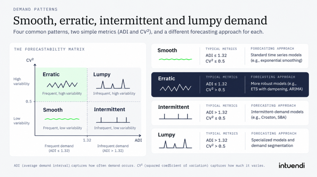
There is no universal level of accuracy that counts as good: it depends on sector, product life cycle and horizon. What you can set is a realistic expectation per quadrant, and judge each SKU against its own quadrant instead of the catalogue average. For a wider view of the options, see our overview of forecasting methods.
| Quadrant | Approach | Realistic accuracy expectation |
|---|---|---|
| Smooth (low ADI, low CV²) | Standard time-series methods such as exponential smoothing, with trend and seasonality where they exist. | Usually the easiest demand pattern to forecast, but accuracy still depends on the data, horizon and model. |
| Erratic (low ADI, high CV²) | The same methods, plus known drivers such as promotions and price changes. Safety stock sized to the swings. | A usable average, but wide error in any single period. Aggregating across weeks or channels narrows it. |
| Intermittent (high ADI, low CV²) | Croston-type methods, which estimate order size and the gap between orders separately. | Period-by-period error stays high because timing is hard to call. Judge it on stock-outs and overstock, and on WAPE over a longer window; pointwise percentage errors are undefined when actual demand is zero. |
| Lumpy (high ADI, high CV²) | Croston-type estimates with caution, or a simple stock rule such as a minimum level, or ordering against confirmed demand. | Usually the hardest demand pattern to forecast. Some of it may remain effectively unpredictable, regardless of the model used. |
That last row is the honest limit. For a lumpy SKU, the best use of your time is often to decide how much buffer you are willing to fund and what a stock-out costs, then stop tuning the forecast. An ABC analysis helps here: a lumpy C item deserves a rule, while a lumpy A item deserves a closer look at its buffer and its supplier terms.
Forecastability in FMCG and retail
Promotions and seasonal products have explainable variability: include known events and external variables rather than treating every spike as noise.
New launches have no sales history, so borrow a starting pattern from similar SKUs and update it as actual demand arrives.
Start with the zero-sale weeks in your order history
The step that changes the result most is the one that is easy to skip: keeping the periods with zero sales. Take the export you already have, compute ADI and CV² for each SKU at your reorder rhythm, and count how many items land above both thresholds. If that lumpy group is a tail of C items, a simple stock rule covers them, and your forecasting effort belongs to the smooth and erratic SKUs. If it includes A items, the question moves from the model to how much buffer you fund and what a stock-out costs on those lines.
That quadrant split is also the most useful thing to bring to us. Our engine combines time-series analysis and machine learning with external variables such as promotions and holidays to generate realistic demand scenarios. Forecasts and reorder suggestions are then turned into SKU-by-SKU decisions by Symphonie, Intuendi’s in-app AI intelligence layer. See how the demand forecasting software connects forecast outputs to planning decisions.
Forecastability describes how predictable demand is, based on its underlying patterns and available information. Forecast accuracy measures how closely a forecast matches actual demand. A product can have relatively predictable demand but poor forecast accuracy because of unsuitable models, data quality issues, or planning processes. Conversely, highly erratic demand may remain difficult to forecast even with a well-designed model. Comparing both helps identify where forecasting improvements are realistic.
There is no universal forecastability score or threshold that works for every SKU. The coefficient of variation (CoV) helps assess relative demand variability, while average demand interval (ADI) can help identify intermittent demand. These measures should be interpreted alongside the forecasting horizon, data quality and business context. A practical test is whether a model consistently outperforms a simple baseline on historical periods excluded from model training.
Not all demand uncertainty can be eliminated, but you can improve how accurately it is measured and forecast. Start by correcting missing data, accounting for stockouts, identifying promotions and distinguishing exceptional orders from recurring demand. Choose an appropriate forecasting level and incorporate relevant demand drivers where available. Then compare forecasting approaches against a simple baseline. These actions improve forecasting decisions, although they do not necessarily make the underlying demand more predictable.
Combine demand forecastability with business importance, such as an ABC classification based on consumption value. Stable, high-value SKUs may be suitable for structured statistical forecasting and regular monitoring, while high-value items with erratic demand often require closer review and scenario-based planning. Lower-value SKUs may benefit from simpler replenishment processes. Inventory policies should also reflect supplier lead times, product criticality, service targets and stockout costs rather than forecastability alone.
Forecast Value Added (FVA) measures whether a forecasting activity improves performance compared with a baseline or the previous step in the forecasting process. Forecastability describes how predictable demand is; FVA evaluates whether forecasting methods, adjustments or reviews actually add value. Comparing forecast errors on consistent out-of-sample periods helps identify useful activities and unnecessary interventions. Tracking FVA by SKU segment can also show where additional forecasting effort is most worthwhile.
