



Ranked by annual consumption value alone, two SKUs can land in class A together even though you would buy them in opposite ways: one sells at a steady rhythm, the other swings week to week. ABC ranks them as equals. Your purchase orders can’t afford to. With a small team, guessing on the volatile one means either empty shelves on a best-seller or cash parked in stock nobody asked for.
Add a second axis, demand variability, and your catalogue splits into nine cells, each with its own policy: strict control where value is high and demand stable, light oversight where little is at stake, extra attention to the forecast where value meets volatility. Refresh the grid as demand shifts and replenishment stays pointed at the SKUs that matter now.
ABC XYZ analysis meaning: what the model is and why ABC alone is not enough
ABC tells you how much money a SKU moves through your business. It says nothing about how hard that SKU is to predict, and that gap is where purchasing decisions go wrong. XYZ analysis closes it by ranking the same catalogue a second time, by how far demand swings around its average.
The two axes are independent, and that is the point. A SKU can be high value and erratic, or cheap and perfectly regular. Planning with spreadsheets tends to blur “important” and “predictable” into one idea. For the value side, our guide to ABC analysis covers the basics. Here we start from the moment you need the second axis.
ABC and XYZ analysis: the logic and formula behind each class
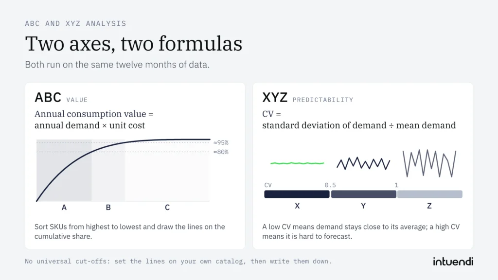
Each axis answers one question with one formula. Both run on the same twelve months of data, so you can build them side by side without a new data source.
ABC classes by annual consumption value
The ABC analysis formula is: annual consumption value = annual demand × unit cost. Sort SKUs from highest to lowest, then draw the A, B and C lines on the cumulative share. The Pareto 80/20 rule is a useful reference for where the lines might fall, but it is a reference only.
This is not revenue, not units sold and not margin. A fast-moving €2 item and a slow €200 item can end up in the same class, and that is exactly what the formula is meant to show you. Where you cut A from B depends on your catalogue, your sector and what you want to protect.
XYZ classes by coefficient of variation
The XYZ analysis formula is the coefficient of variation: CV = standard deviation of demand ÷ mean demand. A low CV means demand stays close to its average (X). A mid-range CV means it varies (Y). A high CV means it is highly variable and hard to forecast (Z).
XYZ measures predictability, never economic value. In a spreadsheet, STDEV.P divided by AVERAGE over your monthly demand gives you the number. Our piece on demand variability goes deeper into what drives it.
As with ABC, there are no universal cut-offs between X, Y and Z. A common starting point is a CV up to 0.5 for X and above 1 for Z. Plot the CVs of your own catalogue, look for natural breaks and set the lines to match your goals. Then write them down, so the next review uses the same rules.
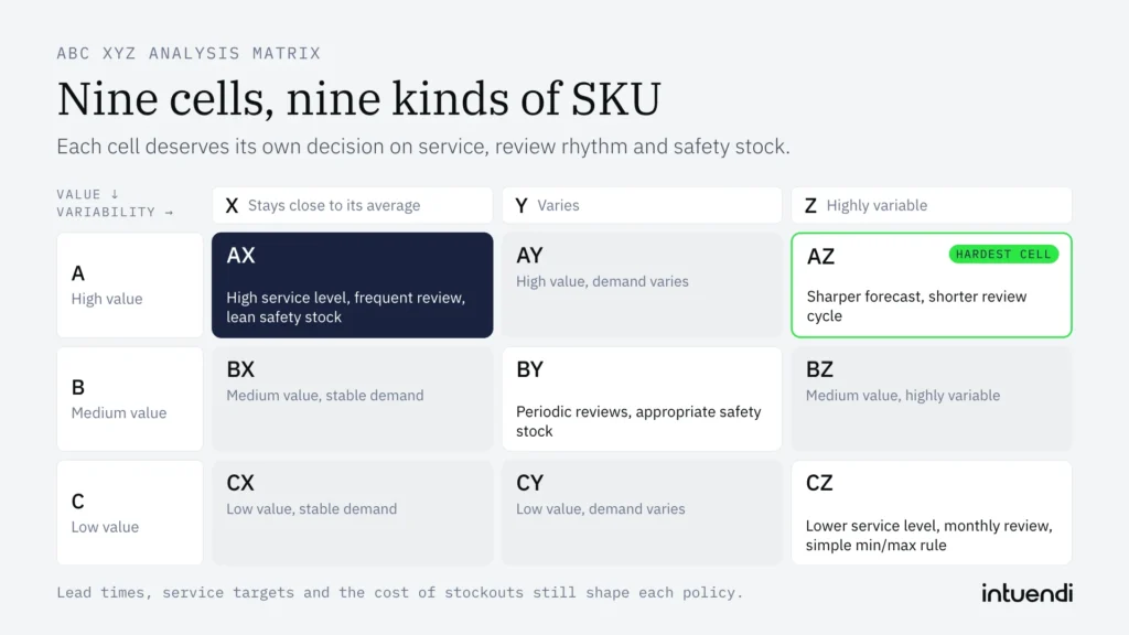
ABC XYZ analysis matrix
Cross the three value classes with the three variability classes and you get the ABC-XYZ matrix: nine cells, AX through CZ. Each cell describes a different kind of SKU, so each deserves its own decision on service, review rhythm and safety stock.
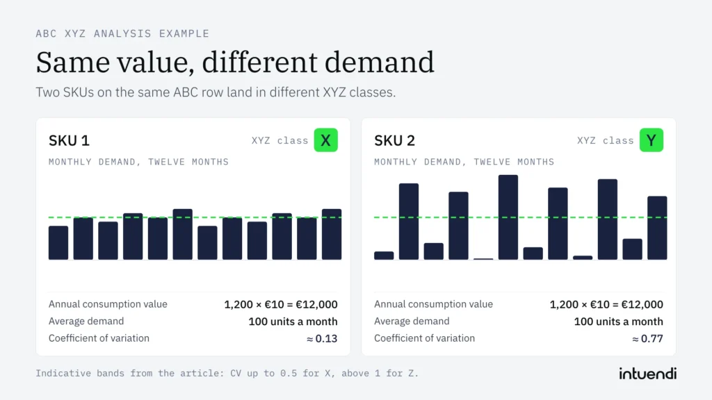
ABC XYZ analysis example
Take two SKUs, both with a unit cost of €10 and 1,200 units sold over twelve months. The annual consumption value is identical: 1,200 × €10 = €12,000. ABC cannot tell them apart.
Now the monthly demand. SKU 1 sells 80, 100, 90, 110, 100, 120, 80, 100, 90, 110, 100, 120 units. SKU 2 sells 20, 180, 40, 160, 0, 200, 30, 170, 10, 190, 50, 150. Both average 100 units a month. SKU 1 has a standard deviation of about 13, so its CV is about 0.13. SKU 2 has a standard deviation of about 77, so its CV is about 0.77.
The value is the same, but SKU 2’s CV is almost six times higher: under the indicative bands used in this article, SKU 1 falls in X and SKU 2 in Y. They land in different cells on the same ABC row, even though their annual consumption value is identical, and they need different policies for service, review rhythm and safety stock.
The inventory policy for each cell
A nine-cell grid only pays off when each cell gets its own rules. Three levers do most of the work: the target service level, the review frequency and the safety stock buffer. Set them cell by cell and you stop applying one blanket policy to a catalogue that behaves in nine different ways.
Start with the corners. AX items (high value, stable demand) deserve a high service level and frequent review, weekly or even continuous. Because demand is predictable, safety stock can stay lean and the target coverage tight, which frees working capital without exposing your best-sellers. CZ items sit at the opposite end: low value, erratic demand. Here a lower service level, a monthly review and a simple min/max rule are usually enough, and for true slow-movers, ordering only on demand is often the cheapest choice.
The hardest cell is AZ, where value meets volatility. Depending on the SKU’s demand pattern, service target and lead time, a high service level can require a larger buffer and tie up substantial cash. Two moves can help keep it under control: a sharper forecast, built on events, promotions and recent actual vs forecast gaps, and a shorter review cycle, so you react before the error compounds. Reducing lead time variability with suppliers can also lower safety stock without changing the service level.
Is ABC XYZ Analysis Right for Your Business?
ABC XYZ analysis is useful when a catalogue contains enough variation in value and demand patterns to justify different replenishment policies. It is less useful when data is sparse, demand is mostly stable, or the cost of maintaining multiple policies outweighs the benefit. Treat the matrix as a decision aid, not an automatic answer: supplier constraints, promotions, stock-outs and business priorities still need planner judgment.
How to run ABC XYZ analysis in Excel, Power BI and Python
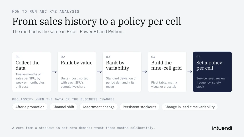
The method is the same in every tool, so start with the data. You need at least twelve months of sales history per SKU, grouped by week or month, plus a unit cost. For the ABC axis, multiply units by cost to get annual consumption value, sort descending, and calculate each SKU’s cumulative share of the total. The common cut-offs are roughly 80% for class A, the next 15% for B and the last 5% for C. For the XYZ axis, divide the standard deviation of period demand by its mean. This gives the coefficient of variation, where a low value means a steady SKU and a high value means a volatile one.
Which tool you choose depends on catalogue size and how often you refresh:
- Excel: Works well up to a few thousand SKUs. Use
AVERAGEandSTDEV.Pacross the monthly columns,SORTBYand a runningSUMfor the cumulative share, andIFSto assign the classes. A pivot table then shows the nine-cell grid in a few clicks. - Power BI: The better fit when the grid has to be shared and refreshed. Power Query cleans and aggregates the sales extract, DAX measures calculate value share and variability, and a matrix visual puts A, B and C against X, Y and Z. Planners and buyers can filter by warehouse or category without touching the formulas.
- Python: Suited to large catalogues and repeatable runs. With pandas,
groupbyaggregates sales per SKU,cumsumbuilds the cumulative share,std() / mean()returns the variability, andpd.crosstabproduces the matrix. The script can be scheduled, so the classification stays current without manual work.
Whichever tool you use, a few choices decide whether the result is usable. Thresholds are not universal, so calibrate the X, Y and Z bands on your own demand profile. Start from the indicative bands given in the XYZ section and adjust them. Treat months with no sales deliberately, because a zero from a stock-out is not the same as zero demand, and it will distort variability if left in as is. New SKUs with 6–12 months of history may support a provisional classification, provided it is reviewed earlier than the standard cycle. SKUs with shorter histories require additional caution and may be better flagged separately until enough reliable demand data is available.
When to reclassify ABC XYZ inventory
Reclassify when your data or your business has changed, not because the calendar says it is a new quarter. Review the grid after a promotion, channel shift, assortment change, persistent stock-outs, or a clear change in lead-time variability. For stable catalogues, an annual review may be enough; volatile categories may need more frequent checks. Use the same thresholds each time, record the reason for a change, and move a SKU only when the new pattern is persistent rather than a one-off spike.
When these update rules are managed manually, they are easy to lose, so the analysis can remain a report instead of reaching replenishment. Intuendi’s AI-powered platform connects to your ERP via API and can support a workflow for reviewing SKU classifications alongside replenishment decisions. The classification rules and review timing still need to be defined against your data and business context.
Start with the A items whose demand won’t sit still
Use the indicative bands above (CV up to 0.5 for X, above 1 for Z) as a starting point, then calibrate them against the gap in your own catalogue. You can check it today. Export twelve months of monthly sales for the SKUs you rank A, divide STDEV.P by AVERAGE for each one, and sort the column from lowest to highest CV.
A clear gap in that sorted column is the second axis showing up in your own catalogue. The A SKUs below it, with the higher CVs, are the ones that need their own decision on service, review rhythm and safety stock. A smooth climb in the CV column means ABC alone may hold for now; a jump with A SKUs on both sides of it means two cells and two policies.
ABC analysis ranks items by value, usually revenue, margin or consumption value. It is based on the Pareto principle (the 80/20 rule): class A holds the few high-value items that need strict control, B is moderate, and C is the long tail of low-value items. XYZ analysis ranks the same items by demand variability, measured with the coefficient of variation. X items have stable, predictable demand, Y items fluctuate moderately, and Z items are erratic or sporadic. ABC tells you which products matter most to your money. XYZ tells you how reliably you can forecast them. Combined, the two give you a more useful basis for purchasing and stocking decisions than either one alone.
AX items have high annual consumption value and stable demand, making them suitable for close forecast monitoring and carefully planned replenishment. BY items have medium value and moderate demand variability, requiring periodic reviews and appropriate safety stock. CZ items have low annual consumption value and irregular demand, but this does not automatically mean keeping minimal or zero stock. Stocking and reorder decisions should also consider product criticality, supplier lead times, service level targets and the cost of stockouts.
At minimum, you need SKU-level sales history for 12–24 months, ideally by week or month. Include units sold, plus unit cost or selling price so you can calculate revenue, margin or consumption value for the ABC ranking. Both classifications must use the same period. Useful extras are stock-out dates (to correct demand that was lost because stock ran out), promotion periods, launch and end-of-life dates, and supplier lead times and minimum order quantities for turning classes into reorder rules. Clean the data first: merge duplicate SKUs, remove returns and one-off B2B orders if they distort demand, and handle new products separately because they lack enough history to be classified reliably.
Yes. For a catalogue of a few hundred to a couple of thousand SKUs, Excel or Google Sheets works well. Build a table with one row per SKU. For ABC, sort by annual revenue, calculate each SKU’s cumulative share of the total, and assign A up to about 80%, B up to about 95%, and C for the rest. For XYZ, put monthly demand in columns and calculate the CV with STDEV.P divided by AVERAGE, then assign X, Y or Z using your thresholds. Join the two labels into a combined code such as AX and summarise with a pivot table. The limits are manual refreshes, version errors and the difficulty of handling seasonality or stock-out correction. Past a certain size, inventory planning software saves time.
ABC XYZ analysis helps small teams focus their limited time and inventory budget on the SKUs that matter most. ABC identifies high-value items, while XYZ highlights demand variability. Together, they help prioritize stock reviews, replenishment decisions and safety stock policies. The appropriate policy for each segment also depends on lead times, service targets and the cost of stockouts.
