



In the sales history of a spare part or long-tail SKU, a zero can mark the week customers wanted the item most. If the shelf was empty, that zero records a stockout, not missing demand, and a model trained on it learns to order less exactly where more stock was needed. Meanwhile a moving average flattens every burst into a thin trickle, and MAPE cannot even be calculated when actual sales are zero.
Plans that forecast slow-movers like best-sellers repeat all three problems. The answer is not a bigger model. Read each zero correctly, consider how often demand appears separately from how much arrives, and judge results by service level and capital tied up, not by one accuracy score. Get that right and your reorder points for sporadic items rest on the same disciplined method as those for fast movers, with buffers sized to their real uncertainty.
What makes demand intermittent: ADI, CV² and why ARIMA falls short
A slow-mover is not a smaller best-seller. Its history is a handful of sales separated by long runs of zeros, and ARIMA and simple exponential smoothing read those zeros as noise around a steady level. The output is a flat, thin forecast for an item that sells either nothing or a whole batch. That forecast is biased: it misreads both how often the item sells and how much is sold when it does.
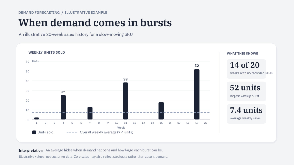
Classifying demand with ADI and CV²
Two numbers sort your catalogue. ADI is the average number of periods between non-zero demands. CV² is the squared coefficient of variation of the non-zero order sizes. Together they place each SKU in one of four quadrants:
- Smooth: frequent sales, stable sizes.
- Erratic: frequent sales, volatile sizes.
- Intermittent: sporadic sales, stable sizes.
- Lumpy: sporadic sales, volatile sizes.
The cut-offs most often used, ADI 1.32 and CV² 0.49, come from Syntetos, Boylan and Croston (2005), “On the categorization of demand patterns”, published in the Journal of the Operational Research Society. They were derived by comparing forecast errors of specific methods, so treat them as a starting point, not a law. You can compute both in a spreadsheet from your sales export in an afternoon.
Forecasting occurrence and size separately
The fix is to forecast two things instead of one: the probability that demand occurs in a period, and its size when it does. Lumpy items are harder because the size part is itself unstable. The picture changes when demand variability starts to dominate.
Before any modelling, check what your zeros mean. A zero in a week when the item was out of stock is censored demand. Leave it in and the model learns that demand is low in exactly the periods you needed inventory. Flag those weeks and either impute them or give them less weight.
Croston, SBA and TSB for intermittent demand
No universal decision tree picks the model for you. The choice depends on history length, known drivers and the stock decision the forecast feeds. Our overview of forecasting methods covers the wider families. Here we stay with the ones built for sparse series.
Croston’s method and its variants: separating occurrence from size
Croston’s method splits the series in two: the non-zero sizes and the intervals between them. It smooths each separately and divides size by interval to get a rate per period. It tends to overstate demand, so SBA (Syntetos-Boylan Approximation) applies a correction factor. Croston only updates when a sale happens, so it keeps forecasting the old rate for a product that has gone quiet. TSB updates the probability of demand every period, so the forecast decays as the zeros pile up. That makes it the better candidate for items drifting toward obsolescence.
A worked Croston example
Take a made-up 12-week series: 0, 0, 5, 0, 0, 0, 3, 0, 0, 0, 0, 4. The non-zero sizes are 5, 3 and 4, averaging 4. The sales fall in weeks 3, 7 and 12. Counting the first interval from the start of the series, the intervals are 3, 4 and 5, averaging 4. The forecast is 4 ÷ 4 = 1 unit per week. (A real implementation smooths with a factor instead of plain averages, but the logic is the same.)
That 1 is a rate, not an order quantity. Over a six-week lead time you expect about six units, but they arrive in lumps, so the rate alone cannot tell you how much buffer to hold; that depends on the service level you target.
When machine learning beats Croston on intermittent demand
Croston-type methods look only at the item’s own sales. Once you have drivers that explain when sales happen, such as promotions, price changes or channel, and enough related SKUs to learn from, machine learning can model the probability of a sale and its size separately. Graph neural networks, which exploit relationships between items, only pay off when data volume and those relationships justify the added complexity. Our piece on machine learning demand forecasting goes deeper on the general approach.
With a short history or a single SKU, ML has nothing to learn from, and a Croston-type baseline, an analogue product or plain judgment is the better call. Test every candidate on the same dataset with the same reproducible evaluation.
Measuring accuracy and turning forecasts into stock decisions
Why MAPE breaks on zeros: MAE and scaled errors
MAPE divides each error by actual demand, so zero actual demand creates division by zero. The metric is undefined; tools may drop those periods or return infinite values. On an intermittent SKU, where zeros dominate the history, this means judging the forecast on only a few non-zero periods. Even a small actual value can distort the result: a two-unit miss against one sale becomes 200%. MAPE can therefore favour forecasts that stay too low and conceal stock-out risk. For SKUs with long runs of zeros, check errors at the right level of aggregation: a weekly miss on one spare part tells you little, while the error over a lead time tells you a lot.
MAE (mean absolute error) averages the absolute gap between actual and forecast in units and handles zero-demand periods without special rules. However, a forecast of zero every period may still achieve a low MAE on a very sparse series because it is usually right. A good score can hide a model that misses the weeks when customers actually buy.
Scaled errors support comparison across SKUs by dividing the error by a benchmark, usually the error of a naive forecast on the same history. MASE (mean absolute scaled error) is the common option: below 1 means the model beats the benchmark; above 1 means it does not. Use metrics that handle zero-demand periods, but note that MASE becomes undefined when an item’s history contains no sales or never varies, because its in-sample naive error is zero. New and dead SKUs need separate treatment. For intermittent demand forecasting, pair MAE or MASE with bias (the signed mean error) to detect systematic over- or under-forecasting. Then check service level, fill rate and inventory coverage: accuracy matters only when it supports availability without tying up unnecessary capital.
From forecast to reorder point
The forecast itself is only the input. What a planner needs is a demand distribution over the lead time, because a single point value hides the risk that sits in the tail. From that distribution you set the safety stock and reorder point for a chosen service level, and the result looks very different from a moving-average estimate. Slow-movers with long lead times often need a higher reorder point than their average sales suggest, while those with short lead times and cheap replenishment can run lean. This is where a target coverage calibrated per SKU class pays off: capital goes where a stock-out costs most, not where a flat rule spreads it.
Close the loop with a routine that compares actuals to the forecast and turns the gap into action:
- Track service level and fill rate per SKU class, not one global accuracy number.
- Monitor inventory value and days of coverage for slow-movers, to catch overstock before it ties up working capital.
- Review bias monthly, and recalibrate parameters when it drifts in one direction.
Done by hand in spreadsheets, this review rarely survives a busy quarter. An AI-powered planning tool such as Intuendi runs the Actual vs Forecast comparison automatically, links it to lead times and target coverage, and returns replenishment suggestions your team can check and approve. The planner stays in control, sees why each quantity was proposed, spends time on exceptions instead of recalculation, and can decide which slow-movers need safety stock and which simply need patience.
Check your zeros before you pick a model
The first check needs only a sales export and a stockout log. Compute ADI and CV² per SKU, flag every zero that fell in an out-of-stock week, and count how many intermittent items you still forecast like best-sellers.
That count shows how large the problem is. To move from analysis to execution, explore Intuendi’s ERP and supply-chain integrations.
No single method wins on every SKU, but Croston-type methods are the usual starting point. Croston’s method forecasts the size of non-zero demand and the interval between demand events separately. The Syntetos-Boylan Approximation (SBA) corrects Croston’s upward bias. TSB (Teunter-Syntetos-Babai) updates the probability of demand every period, so it handles items that are becoming obsolete better. In practice, classify SKUs by demand pattern first, then test two or three methods on your own history. Choose the one with the lowest error on a hold-out sample, using metrics suited to zero-heavy data. Treat a slow mover as its own type of series, not a smaller version of a best seller.
Moving averages and standard exponential smoothing assume demand is continuous, so they treat zeros as ordinary low values. On intermittent series, the forecast drops after each zero period and jumps after each sale. It never matches the real pattern, which is either zero or a lump. The result is a low, flat forecast that is almost never correct in any single period. It tends to under-forecast just before a sale and over-forecast just after one. Croston-type methods avoid this by modeling demand size and demand interval separately. This gives a more stable estimate of average demand per period.
First, separate true zeros from false zeros. A true zero means customers did not want the product. A false zero means a stockout, a data gap, or a delisting hid real demand. Stockouts censor demand, so flag those periods and either impute demand or down-weight them. Do not delete genuine zeros, because they carry information about demand frequency. Then use a method built for zeros, such as Croston, SBA, or TSB, or a model that predicts probability of demand plus size of demand. If weekly data is mostly zeros, try aggregating to monthly buckets, or forecast over the lead time rather than period by period.
Sometimes, but not automatically. Machine learning can help when you have many related SKUs and useful drivers such as promotions, price, or customer orders. In those cases, a global model trained across items can learn shared patterns. For short, noisy series with no external signals, Croston, SBA, or TSB often match or outperform complex models and are easier to explain. Whichever you choose, the model should handle zero-heavy data, for example by predicting the probability of demand and the size of demand. Compare any ML model against a Croston-type baseline on a hold-out period, and use it only if it improves both accuracy and inventory outcomes.
For items with sporadic demand, traditional safety stock formulas based on normal demand distributions may be unreliable. Instead, estimate demand during replenishment lead time using historical demand patterns, simulations or a suitable statistical distribution. Set safety stock according to the desired service level, lead time variability and cost of a stockout. Review the result against actual availability and inventory holding costs, especially for slow-moving or high-value SKUs.
