

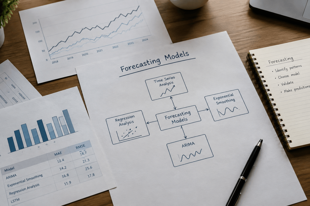

Choosing a forecasting model is not a contest to find the most sophisticated algorithm.
For a demand planner, the useful question is whether the model reflects the way demand behaves at the horizon where a decision has to be made. A model can look excellent on historical data and still be operationally weak if it misses a promotion, struggles with intermittent demand, or performs poorly over the lead-time window that actually drives a purchase order.
There is no forecasting model that is best for every product, channel, location, and planning horizon. The right choice depends on the data you have, the pattern you are trying to forecast, the information available about future demand drivers, and the cost of getting the forecast wrong.
This guide explains the main forecasting model families, where they tend to fit, how to compare them fairly, and when the real problem is no longer choosing a model but operating a forecasting process at scale.
What is a forecasting model?
A forecasting model is a mathematical or statistical representation used to estimate future values from the information available today.
Depending on the approach, that information may include:
- historical demand;
- trend and seasonality;
- calendar effects;
- promotions and prices;
- external variables;
- relationships between products, locations, or channels.
A forecasting method is broader. It describes how a forecast is produced, while the full forecasting process also includes data preparation, parameter estimation, validation, human review, monitoring, and the way the forecast is ultimately used.
That distinction matters in practice. A technically sound model can still produce poor planning outcomes if it is trained on weak data, validated at the wrong horizon, or disconnected from the inventory and purchasing decisions that follow.
The main types of forecasting models
The easiest way to compare forecasting models is not by asking which one is “more advanced”, but by asking what kind of demand pattern each is designed to handle.
1. Qualitative and judgment-based forecasting
When relevant historical data are unavailable or too limited to support a useful quantitative model, judgment becomes part of the forecast.
This is common with:
- new product launches;
- entry into a new market;
- major assortment changes;
- events with no useful historical precedent.
Inputs can include expert judgment, market research, commercial assumptions, customer feedback, and analog products.
The important part is to make the assumptions visible. Judgmental forecasts are useful precisely because history is weak, but that also makes them harder to reproduce and easier to bias if the reasoning behind them is not documented.
2. Naive methods and moving averages
Simple methods are useful benchmarks and, in some cases, useful forecasts in their own right.
A naive forecast may use the latest observed value, while a moving average smooths recent observations to reduce short-term noise.
These approaches can work reasonably well when demand is relatively stable, but they are less suited to series with pronounced trend, seasonality, promotional effects, or sudden structural changes.
Their main value is not that they are unsophisticated. It is that every more complex model should be able to justify why it performs better than a credible baseline.
3. Exponential smoothing models
Exponential smoothing gives more weight to recent observations while allowing older data to contribute progressively less.
Different forms can represent:
- level;
- trend;
- damped trend;
- seasonality.
This makes exponential smoothing useful for many business time series where these components are visible and reasonably persistent.
The model family is especially valuable because it can provide a strong balance between forecast quality, speed, and interpretability.
4. ARIMA and seasonal ARIMA models
ARIMA models focus on the statistical dependence between current and past values of a series.
They can model autocorrelation and use differencing to handle non-stationary patterns. Seasonal extensions can also represent recurring seasonal structures.
ARIMA can be effective when the historical series contains stable statistical patterns, but it does not automatically know that a price promotion, marketing campaign, or supplier event is about to happen. When those factors matter, they need to be incorporated through additional predictors or another modeling approach.
5. Regression and causal forecasting
Regression models are useful when demand is related to variables that can be observed or reasonably specified for the forecast period.
Examples include:
- price;
- discount depth;
- promotions;
- holidays;
- marketing activity;
- weather;
- economic indicators.
This can be more informative than relying on the demand history alone, especially when known business events materially change customer behavior.
The important caveat is that future values of those predictors must either be known, forecast separately, or represented through scenarios. A causal model is only as useful as the assumptions made about the variables driving it.
6. Intermittent-demand models
Some products do not sell every day, week, or month. Demand arrives in bursts separated by zero-demand periods.
This pattern is common with:
- spare parts;
- specialty items;
- long-tail SKUs;
- low-frequency components.
Treating these series like continuous high-volume demand can produce misleading forecasts. Methods designed for intermittent demand, such as Croston-type approaches, separate the size of non-zero demand from the interval between demand occurrences.
For inventory teams, this distinction matters because a slow mover is not simply a smaller version of a best seller.
7. Machine-learning and deep-learning forecasting
Machine-learning models can be useful when forecasting requires many variables, nonlinear relationships, or information shared across large collections of products and locations.
Depending on the setup, models can learn from combinations of:
- historical sales;
- calendar effects;
- promotions;
- price;
- channel behavior;
- product attributes;
- external variables;
- patterns shared across related series.
That does not make machine learning automatically more accurate.
More flexible models can also require more data, stronger feature engineering, more disciplined validation, and more monitoring. A complex model that performs well in training but fails on future periods is still a poor forecasting model.
The relevant comparison is always out-of-sample performance at the horizon that matters to the business.
Which forecasting model should you choose?
There is no universal decision tree, but this framework is a practical starting point.
| Demand situation | Models or approaches worth testing | What to watch |
| Very limited history | Expert judgment, analogs, simple benchmarks | Assumptions and bias |
| Relatively stable demand | Naive methods, moving averages, simple exponential smoothing | Sudden trend or regime changes |
| Trend and/or seasonality | Exponential smoothing, ARIMA/SARIMA | Changing seasonal patterns |
| Promotions or known external drivers | Regression, dynamic regression, machine learning | Quality and future availability of predictors |
| Intermittent / many zero-demand periods | Croston-type or other intermittent-demand approaches | Whether zeros are genuine demand gaps or stockouts |
| Many related SKU/location series | Machine learning, hierarchical/grouped approaches, ensembles | Scalability, coherence, explainability |
| New products | Judgment, analog products, product attributes, market inputs | Lack of true historical demand |
The point is not to choose a model from the table and stop.
The point is to define a credible set of candidates and test them against the decision the forecast is meant to support.
How to compare forecasting models without fooling yourself
Start with a benchmark
A sophisticated model should be compared with a simple baseline.
If a complex model cannot reliably outperform a naive or seasonal benchmark on future-like data, the extra complexity may not be buying you anything.
Validate on data the model has not seen
Good fit on historical training data is not evidence of good forecasting.
Forecasts should be evaluated on later periods that were not used to fit the model. Rolling-origin or time-series cross-validation is particularly useful because it repeatedly tests how the model would have performed as time moved forward.
Match the evaluation horizon to the decision
A model can be excellent one day ahead and weak six weeks ahead.
That distinction matters if a supplier lead time is six weeks.
The relevant forecast horizon should reflect the planning decision: replenishment cycle, supplier lead time, budgeting period, production horizon, or another operational window.
Do not rely on one accuracy metric blindly
MAE, RMSE, percentage errors, scaled errors, and bias each reveal different aspects of forecast performance.
The right metric also depends on the data. Percentage metrics, for example, become problematic when actual demand can be zero or close to zero.
For planning, statistical accuracy should also be connected to the business consequence of the error. Under-forecasting a critical best seller and over-forecasting a low-value slow mover may have very different costs.
Evaluate different product groups separately
Best sellers, seasonal items, new products, and long-tail SKUs do not necessarily deserve the same forecasting logic.
A single average accuracy number across an entire catalog can hide poor performance exactly where the business risk is highest.
Keep monitoring after deployment
Model selection is not a one-time event.
Demand changes, product mixes evolve, promotions become more aggressive, channels shift, and new data become available. Forecast performance should be monitored against actual demand so the process can detect drift and decide when a model needs to be recalibrated, retrained, or replaced.
Building forecasting models in Python, Excel, and Power BI
Choosing a model on paper is only half the job. At some point you need to build it, test it against real numbers, and hand it to someone who has to act on it by Monday morning. Python is a flexible option: libraries such as statsmodels, Prophet, and scikit-learn support different forecasting workflows, including ARIMA, exponential smoothing, and regression-based models, while holdout or rolling-origin evaluation can be used before deployment. The trade-off is clear: you get precision and control, but you also need someone to maintain the code as the data and business requirements change.
Excel remains useful for many planning teams, particularly for smaller datasets and transparent scenario checks. It’s fast for moving averages, simple exponential smoothing, or a quick linear trend on a handful of SKUs, and it’s the format most stakeholders already trust. The ceiling shows up quickly, though: once you’re forecasting hundreds of SKUs across multiple warehouses, or trying to layer in promotions and lead times, spreadsheets turn into a maintenance burden that eats the time you meant to save.
Power BI is primarily a reporting and visualization tool. You can also add forecasting and machine-learning capabilities through built-in features, Python or R integration, and Microsoft Fabric services, depending on your setup. Many teams end up combining the three: Python for the modeling logic, Excel for quick checks or ad hoc scenarios, Power BI for reporting the results to people who need the number, not the math behind it.
The real question isn’t which tool wins — it’s where each one stops paying off:
- Python for building and testing models at scale, especially with irregular seasonality or many variables
- Excel for fast, low-volume forecasts and one-off validation
- Power BI for surfacing forecast accuracy and trend shifts to planners and buyers
- All three for prototyping, before deciding whether the volume of SKUs justifies something more automated
That last point is where most teams eventually hit a wall. A forecasting model that works for fifty SKUs in a spreadsheet doesn’t scale to five thousand without breaking someone’s week. That’s often the moment to consider a system that recalculates forecasts at SKU and channel level, highlights potential demand shifts for review, and supports replenishment decisions alongside reporting. The model matters, but so does whether someone still has to rebuild it by hand every time the data changes.
A forecasting model is an input for the final decision
Forecast accuracy matters, but supply-chain teams do not forecast for the sake of producing a better number.
They forecast because another decision follows.
A demand forecast can influence:
- how much inventory to hold;
- where stock should be positioned;
- what to reorder;
- how much to reorder;
- when to place an order;
- how much working capital will be committed;
- where stockout or excess-inventory risk is increasing.
That is why model evaluation should not stop at an accuracy leaderboard.
The relevant question is whether the forecast improves the planning decision that comes next.
How Intuendi connects forecasting to planning
Intuendi is built around the idea that the forecast should feed the next decision.
The platform can analyze demand across products, SKUs, channels, and locations while accounting for factors such as historical demand, trends, seasonality, promotions, and calendar events.
That demand view then connects with inventory and replenishment planning, where factors such as inventory position, supplier lead times, budgets, logistics constraints, transfers, and service-level objectives may also matter depending on the use case and configuration.
The result is not simply another forecast chart.
It is a planning workflow designed to help teams move from:
data → forecast → inventory risk → replenishment decision
If your team already knows how to build forecasts but spends too much time maintaining spreadsheets, reconciling models, or translating the output into purchase decisions, that is usually a more important signal than the number of forecasting algorithms available.
Explore Intuendi’s demand forecasting software
There is no universally most accurate model. Performance depends on the demand pattern, available data, forecast horizon, external variables, and how the model is validated. The useful approach is to compare candidate models on unseen data at the horizon that matters to the business.
There is no single minimum that applies to every series. You need enough relevant history to expose the patterns the model is expected to learn. A seasonal product may require enough observations to understand recurring seasonal behavior, while a new product may require analogs, market inputs, or expert judgment because its own history does not exist.
No. Machine learning can be valuable when there are many related series, nonlinear relationships, and useful external variables. Simpler statistical methods can still perform extremely well on many time series and are often easier to maintain and interpret. The choice should be made through out-of-sample evaluation, not model prestige.
Yes. Excel is useful for simple forecasts, benchmarks, scenarios, and smaller planning problems. The challenge is maintainability when the number of products, locations, variables, refreshes, and collaborators increases.
When a product has little or no history, teams typically combine judgment with information from comparable products, product attributes, market research, commercial assumptions, and early sales data. The forecast should be updated quickly as real demand becomes observable.
There is no universal schedule. Models should be monitored against actual demand and reviewed when performance deteriorates, demand behavior changes, the assortment changes materially, or new predictive information becomes available.
Because a forecast is normally an input into another decision. In supply chain planning, the business consequence may be a stockout, excess inventory, an unnecessary purchase order, or working capital tied up in the wrong products. A useful forecasting process therefore evaluates both statistical performance and the quality of the operational decisions it supports.
